

We live in the world of sounds: Pleasant and annoying, low and high, quiet and loud, they impact our mood and our decisions. Our brains are constantly processing sounds to give us important information about our environment. But acoustic signals can tell us even more if analyze them using modern technologies.
Today, we have AI and machine learning to extract insights, inaudible to human beings, from speech, voices, snoring, music, industrial and traffic noise, and other types of acoustic signals. In this article, we’ll share what we’ve learned when creating AI-based sound recognition solutions for healthcare projects.
Particularly, we’ll explain how to obtain audio data, prepare it for analysis, and choose the right ML model to achieve the highest prediction accuracy. But first, let’s go over the basics: What is the audio analysis, and what makes audio data so challenging to deal with.
What is audio analysis?
Audio analysis is a process of transforming, exploring, and interpreting audio signals recorded by digital devices. Aiming at understanding sound data, it applies a range of technologies, including state-of-the-art deep learning algorithms. Audio analysis has already gained broad adoption in various industries, from entertainment to healthcare to manufacturing. Below we’ll give the most popular use cases.
Speech recognition
Speech recognition is about the ability of computers to distinguish spoken words with natural language processing techniques. It allows us to control PCs, smartphones, and other devices via voice commands and dictate texts to machines instead of manual entering. Siri by Apple, Alexa by Amazon, Google Assistant, and Cortana by Microsoft are popular examples of how deeply the technology has penetrated into our daily lives.
Voice recognition
Voice recognition is meant to identify people by the unique characteristics of their voices rather than to isolate separate words. The approach finds applications in security systems for user authentication. For instance, Nuance Gatekeeper biometric engine verifies employees and customers by their voices in the banking sector.
Music recognition
Music recognition is a popular feature of such apps as Shazam that helps you identify unknown songs from a short sample. Another application of musical audio analysis is genre classification: Say, Spotify runs its proprietary algorithm to group tracks into categories (their database holds more than 5,000 genres)
Environmental sound recognition
Environmental sound recognition focuses on the identification of noises around us, promising a bunch of advantages to automotive and manufacturing industries. It’s vital for understanding surroundings in IoT applications.
Systems like Audio Analytic ‘listen’ to the events inside and outside your car, enabling the vehicle to make adjustments in order to increase a driver’s safety. Another example is SoundSee technology by Bosch that can analyze machine noises and facilitate predictive maintenance to monitor equipment health and prevent costly failures.
Healthcare is another field where environmental sound recognition comes in handy. It offers a non-invasive type of remote patient monitoring to detect events like falling. Besides that, analysis of coughing, sneezing, snoring, and other sounds can facilitate pre-screening, identifying a patient's status, assessing the infection level in public spaces, and so on.
A real-life use case of such analysis is Sleep.ai which detects teeth grinding and snoring sounds during sleep. The solution created by AltexSoft for a Dutch healthcare startup helps dentists identify and monitor bruxism to eventually understand the causes of this abnormality and treat it.
No matter what type of sounds you analyze, it all starts with an understanding of audio data and its specific characteristics.
What is audio data?
Audio data represents analog sounds in a digital form, preserving the main properties of the original. As we know from school lessons in physics, a sound is a wave of vibrations traveling through a medium like air or water and finally reaching our ears. It has three key characteristics to be considered when analyzing audio data — time period, amplitude, and frequency.
Time period is how long a certain sound lasts or, in other words, how many seconds it takes to complete one cycle of vibrations.
Amplitude is the sound intensity measured in decibels (dB) which we perceive as loudness.
Frequency measured in Hertz (Hz) indicates how many sound vibrations happen per second. People interpret frequency as low or high pitch.
While frequency is an objective parameter, the pitch is subjective. The human hearing range lies between 20 and 20,000 Hz. Scientists claim that most people perceive as low pitch all sounds below 500 Hz — like the plane engine roar. In turn, high pitch for us is everything beyond 2,000 Hz (for example, a whistle.)
Audio data file formats
Similar to texts and images, audio is unstructured data meaning that it’s not arranged in tables with connected rows and columns. Instead, you can store audio in various file formats like
- WAV or WAVE (Waveform Audio File Format) developed by Microsoft and IBM. It’s a lossless or raw file format meaning that it doesn’t compress the original sound recording;
- AIFF (Audio Interchange File Format) developed by Apple. Like WAV, it works with uncompressed audio;
- FLAC (Free Lossless Audio Codec) developed by Xiph.Org Foundation that offers free multimedia formats and software tools. FLAC files are compressed without losing sound quality.
- MP3 (mpeg-1 audio layer 3) developed by the Fraunhofer Society in Germany and supported globally. It’s the most common file format since it makes music easy to store on portable devices and send back and forth via the Internet. Though mp3 compresses audio, it still offers an acceptable sound quality.
We recommend using aiff and wav files for analysis as they don’t miss any information present in analog sounds. At the same time, keep in mind that neither of those and other audio files can be fed directly to machine learning models. To make audio understandable for computers, data must undergo a transformation.
Audio data transformation basics to know
Before diving deeper into the processing of audio files, we need to introduce specific terms, that you will encounter at almost every step of our journey from sound data collection to getting ML predictions. It’s worth noting that audio analysis involves working with images rather than listening.
A waveform is a basic visual representation of an audio signal that reflects how an amplitude changes over time. The graph displays the time on the horizontal (X) axis and the amplitude on the vertical (Y) axis but it doesn’t tell us what’s happening to frequencies.
An example of a waveform. Source: Audio Singal Processing for Machine Learning
A spectrum or spectral plot is a graph where the X-axis shows the frequency of the sound wave while the Y-axis represents its amplitude. This type of sound data visualization helps you analyze frequency content but misses the time component.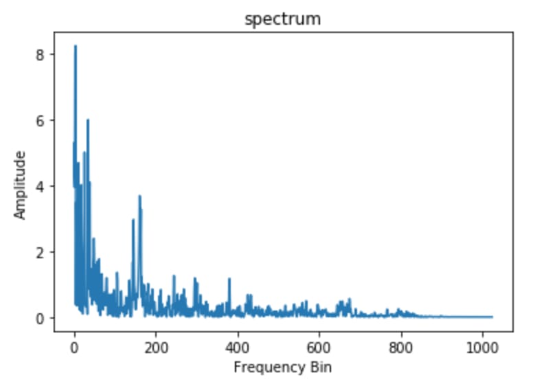
An example of a spectrum plot. Source: Analytics Vidhya
A spectrogram is a detailed view of a signal that covers all three characteristics of sound. You can learn about time from the x-axis, frequencies from the y-axis, and amplitude from color. The louder the event the brighter the color, while silence is represented by black. Having three dimensions on one graph is very convenient: it allows you to track how frequencies change over time, examine the sound in all its fullness, and spot various problem areas (like noises) and patterns by sight.
An example of a spectrogram. Source: iZotope
A mel spectrogram where mel stands for melody is a type of spectrogram based on the mel scale that describes how people perceive sound characteristics. Our ear can distinguish low frequencies better than high frequencies. You can check it yourself: Try to play tones from 500 to 1000 Hz and then from 10,000 to 10,500 Hz. The former frequency range would seem much broader than the latter, though, in fact, they are the same. The mel spectrogram incorporates this unique feature of human hearing, converting the values in Hertz into the mel scale. This approach is widely used for genre classification, instrument detection in songs, and speech emotion recognition.
An example of a mel spectrogram. Source: Devopedia
The Fourier transform (FT) is a mathematical function that breaks a signal into spikes of different amplitudes and frequencies. We use it to convert waveforms into corresponding spectrum plots to look at the same signal from a different angle and perform frequency analysis. It’s a powerful instrument to understand signals and troubleshooting errors in them.
The Fast Fourier Transform (FFT) is the algorithm computing the Fourier transform.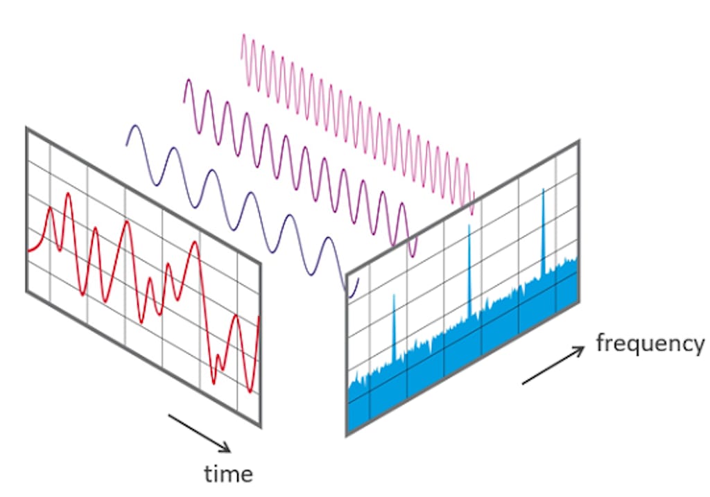
Applying FFT to view the same signal from time and frequency perspectives. Source: NTi Audio
The short-time Fourier transform (STFT) is a sequence of Fourier transforms converting a waveform into a spectrogram.
Audio analysis software
Of course, you don’t need to perform transformations manually. Neither need you to understand the complex mathematics behind FT, STFT, and other techniques used in audio analysis. All these and many other tasks are done automatically by audio analysis software that in most cases supports the following operations:
- import audio data
- add annotations (labels),
- edit recordings and split them into pieces,
- remove noise,
- convert signals into corresponding visual representations (waveforms, spectrum plots, spectrograms, mel spectrograms),
- do preprocessing operations,
- analyze time and frequency content,
- extract audio features and more.
The most advanced platforms also allow you to train machine learning models and even provide you with pre-trained algorithms.
Here is the list of the most popular tools used in audio analysis.
Audacity is a free and open-source audio editor to split recordings, remove noise, transform waveforms to spectrograms, and label them. Audacity doesn’t require coding skills. Yet, its toolset for audio analysis is not very sophisticated. For further steps, you need to load your dataset to Python or switch to a platform specifically focusing on analysis and/or machine learning.
Labeling of audio data in Audacity. Source: Towards Data Science
Tensorflow-io package for preparation and augmentation of audio data lets you perform a wide range of operations — noise removal, converting waveforms to spectrograms, frequency, and time masking to make the sound clearly audible, and more. The tool belongs to the open-source TensorFlow ecosystem, covering end-to-end machine learning workflow. So, after preprocessing you can train an ML model on the same platform.
Torchaudio is an audio processing library for PyTorch. It offers several tools for handling and transforming audio data. It supports various audio formats and provides essential data loading and preprocessing capabilities.
Librosa is an open-source Python library that has almost everything you need for audio and music analysis. It enables displaying characteristics of audio files, creating all types of audio data visualizations, and extracting features from them, to name just a few capabilities.
Audio Toolbox by MathWorks offers numerous instruments for audio data processing and analysis, from labeling to estimating signal metrics to extracting certain features. It also comes with pre-trained machine learning and deep learning models that can be used for speech analysis and sound recognition.
Audio data analysis steps
Now that we have a basic understanding of sound data, let’s take a glance at the key stages of the end-to-end audio analysis project.
- Obtain project-specific audio data stored in standard file formats.
- Prepare data for your machine learning project, using software tools
- Extract audio features from visual representations of sound data.
- Select the machine learning model and train it on audio features.
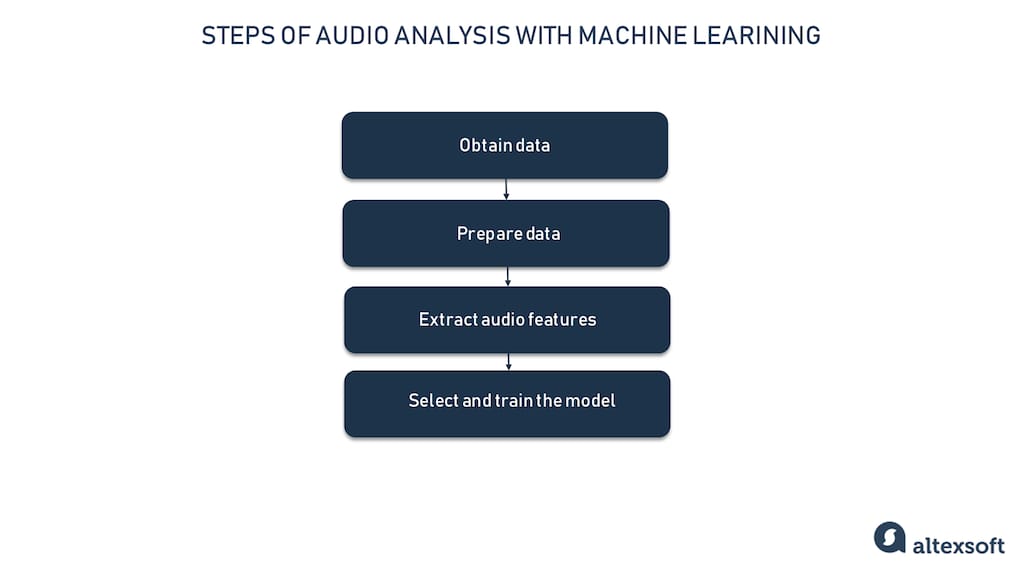
Steps of audio analysis with machine learning
Voice and sound data acquisition
You have three options to obtain data to train machine learning models: use free sound libraries or audio datasets, purchase it from data providers, or collect it involving domain experts.
Free data sources
There are a lot of such sources out there on the web. But what we do not control in this case is data quality and quantity, and the general approach to recording.
Sound libraries are free audio pieces grouped by theme. Sources like Freesound and BigSoundBank offer voice recordings, environment sounds, noises, and honestly all kinds of stuff. For example, you can find the soundscape of the applause, and the set with skateboard sounds.
The most important thing is that sound libraries are not specifically prepared for machine learning projects. So, we need to perform extra work on set completion, labeling, and quality control.
Audio datasets are, on the contrary, created with particular machine learning tasks in mind. For instance, the Bird Audio Detection dataset by the Machine Listening Lab has more than 7,000 excerpts collected during bio-acoustics monitoring projects. Another example is the ESC-50: Environmental Sound Classification dataset, containing 2,000 labeled audio recordings. Each file is 5 seconds long and belongs to one of the 50 semantical classes organized in five categories.
One of the largest audio data collections is AudioSet by Google. It includes over 2 million human-labeled 10-second sound clips, extracted from YouTube videos. The dataset covers 632 classes, from music and speech to splinter and toothbrush sounds.
Commercial datasets
Commercial audio sets for machine learning are definitely more reliable in terms of data integrity than free ones. We can recommend ProSoundEffects selling datasets to train models for speech recognition, environmental sound classification, audio source separation, and other applications. In total, the company has 357,000 files recorded by experts in film sound and classified into 500+ categories.
But what if the sound data you’re looking for is way too specific or rare? What if you need full control of the recording and labeling? Well, then better do it in a partnership with reliable specialists from the same industry as your machine learning project.
Expert datasets
When working with Sleep.ai, our task was to create a model capable of identifying grinding sounds that people with bruxism typically make during sleep. Clearly, we needed special data, not available through open sources. Also, the data reliability and quality had to be the best so we could get trustworthy results.
To obtain such a dataset, the startup partnered with sleep laboratories, where scientists monitor people while they are sleeping to define healthy sleep patterns and diagnose sleep disorders. Experts use various devices to record brain activity, movements, and other events. For us, they prepared a labeled data set with about 12,000 samples of grinding and snoring sounds.
Audio data preparation
In the case of Sleep.io, our team skipped this step entrusting sleep experts with the task of data preparation for our project. The same relates to those who buy annotated sound collections from data providers. But if you have only raw data meaning recordings saved in one of the audio file formats you need to get them ready for machine learning.
Audio data labeling
Data labeling or annotation is about tagging raw data with correct answers to run supervised machine learning. In the process of training, your model will learn to recognize patterns in new data and make the right predictions, based on the labels. So, their quality and accuracy are critical for the success of ML projects.
Though labeling suggests assistance from software tools and some degree of automation, for the most part, it’s still performed manually, by professional annotators and/or domain experts. In our bruxism detection project, sleep experts listened to audio recordings and mark them with grinding or snoring labels.
Learn more about approaches to annotation from our article How to Organize Data Labeling for Machine Learning
Audio data preprocessing
Besides enriching data with meaningful tags, we have to preprocess sound data to achieve better prediction accuracy. Here are the most basic steps for speech recognition and sound classification projects.
Framing means cutting the continuous stream of sound into short pieces (frames) of the same length (typically, of 20-40 ms) for further segment-wise processing.
Windowing is a fundamental audio processing technique to minimize spectral leakage — the common error that results in smearing the frequency and degrading the amplitude accuracy. There are several window functions (Hamming, Hanning, Flat Top, etc) applied to different types of signals, though the Hanning variation works well for 95 percent of cases.
Basically, all windows do the same thing: reduce or smooth the amplitude at the start and the end of each frame while increasing it at the center to preserve the average value.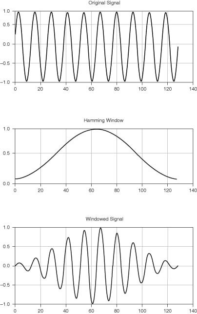
The signal waveform before and after windowing. Source: National Instruments
Overlap-add (OLA) method prevents losing vital information that can be caused by windowing. OLA provides 30-50 percent overlap between adjacent frames, allowing to modify them without the risk of distortion. In this case, the original signal can be accurately reconstructed from windows.
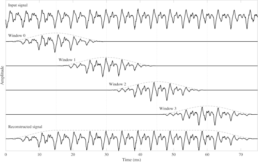
An example of windowing with overlapping. Source: Aalto University Wiki
Learn more about the preprocessing stage and techniques it uses from our article Preparing Your Data For Machine Learning and the video below.

Data preparation explained
Feature extraction
Audio features or descriptors are properties of signals, computed from visualizations of preprocessed audio data. They can belong to one of three domains
- time domain represented by waveforms,
- frequency domain represented by spectrum plots, and
- time and frequency domain represented by spectrograms.
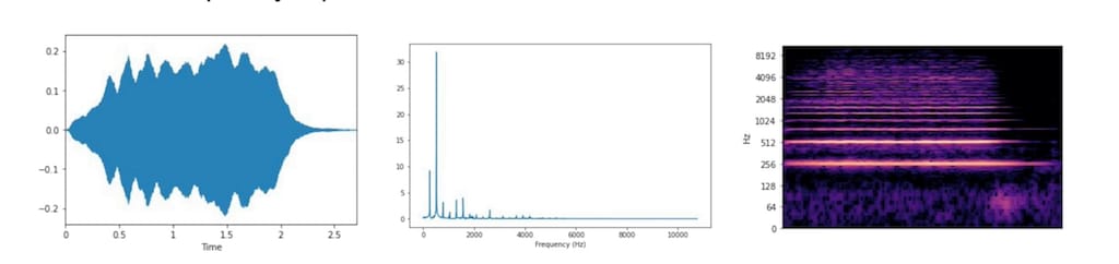
Audio data visualization: waveform for time domain, spectrum for frequency domain, and spectrogram for time-and-frequency domain. Source: Types of Audio Features for ML
Time-domain features
As we mentioned before, time domain or temporal features are extracted directly from original waveforms. Notice that waveforms don't contain much information on how the piece would really sound. They indicate only how the amplitude changes with time. In the image below we can see that the air condition and siren waveforms look alike, but surely those sounds would not be similar.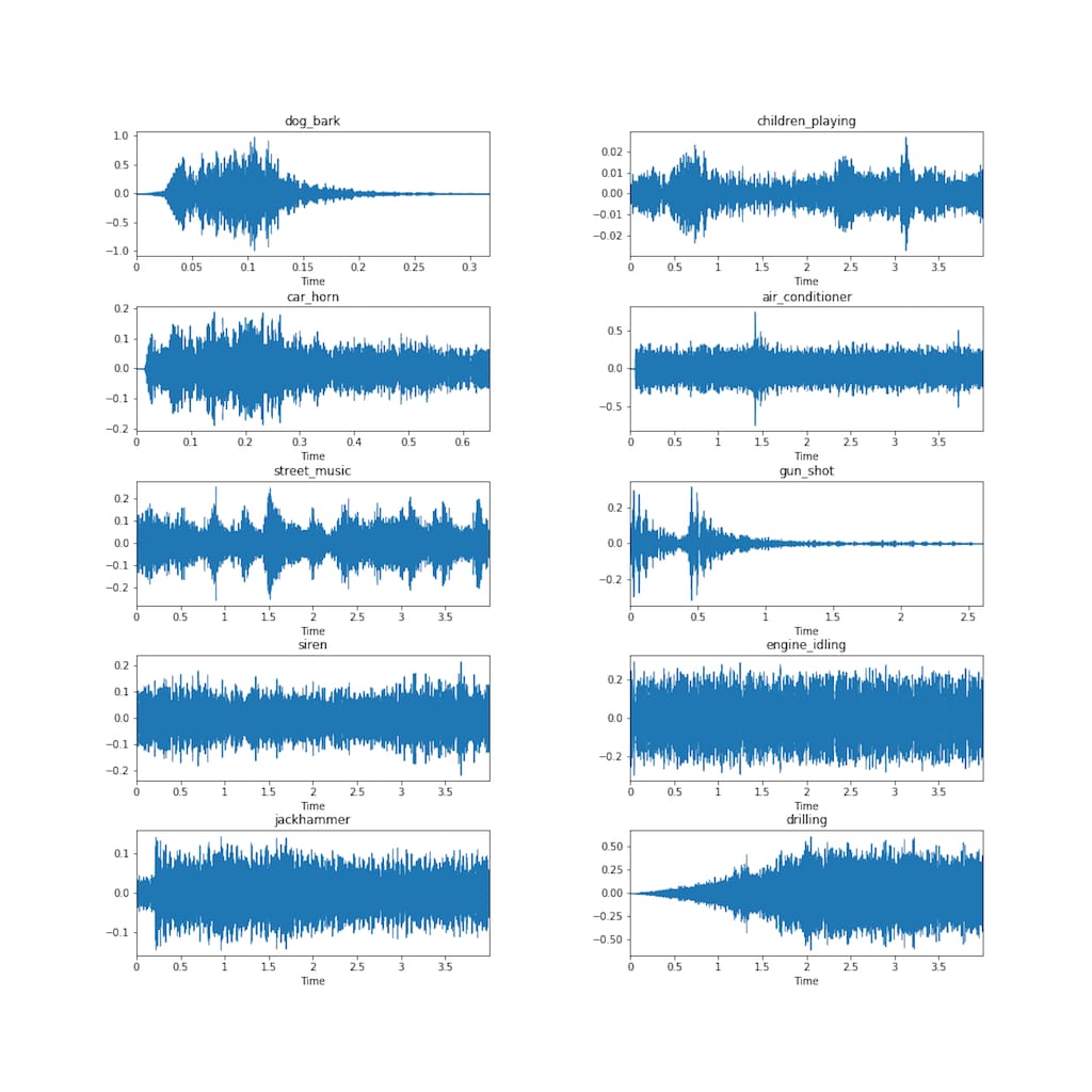
Waveforms examples. Source: Towards Data Science
Now let’s move to some key features we can draw from waveforms.
Amplitude envelope (AE) traces amplitude peaks within the frame and shows how they change over time. With AE, you can automatically measure the duration of distinct parts of a sound (as shown in the picture below). AE is widely used for the onset detection to indicate when a certain signal starts, and for music genre classification.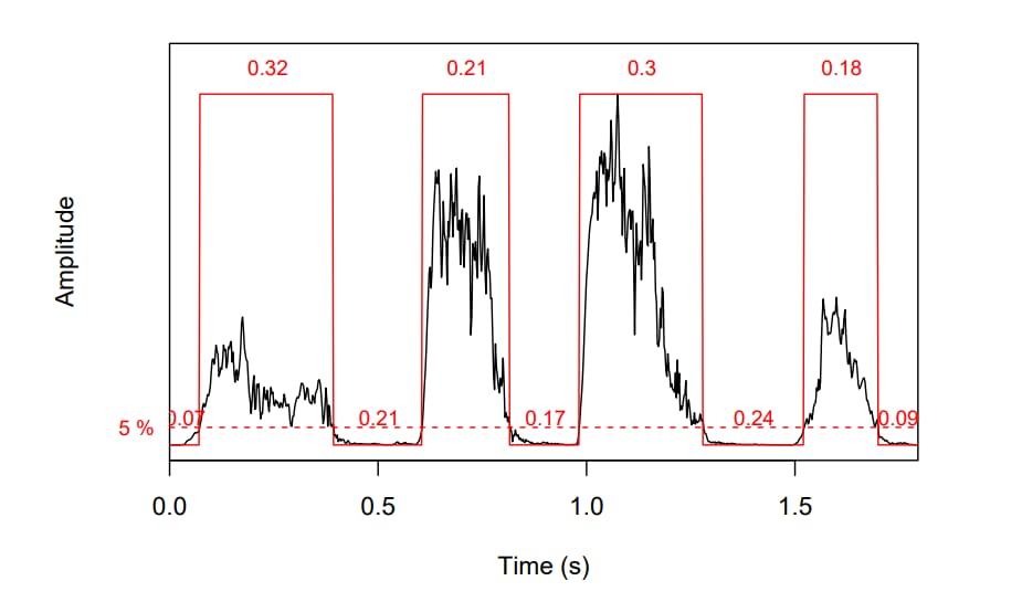
The amplitude envelope of a tico-tico bird singing. Source: Seewave: Sound Anaysis principles
Short-time energy (STE) shows the energy variation within a short speech frame.
It’s a powerful tool to separate voiced and unvoiced segments.
Root mean square energy (RMSE) gives you an understanding of the average energy of the signal. It can be computed from a waveform or a spectrogram. In the first case, you’ll get results faster. Yet, a spectrogram provides a more accurate representation of energy over time. RMSE is particularly useful for audio segmentation and music genre classification.
Zero-crossing Rate (ZCR) counts how many times the signal wave crosses the horizontal axis within a frame. It’s one of the most important acoustic features, widely used to detect the presence or absence of speech, and differentiate noise from silence and music from speech.
Frequency domain features
Frequency-domain features are more difficult to extract than temporal ones as the process involves converting waveforms into spectrum plots or spectrograms using FT or STFT. Yet, it’s the frequency content that reveals many important sound characteristics invisible or hard to see in the time domain.
The most common frequency domain features include
- mean or average frequency,
- median frequency when the spectrum is divided into two regions with equal amplitude,
- signal-to-noise ratio (SNR) comparing the strength of desired sound against the background nose,
- band energy ratio (BER) depicting relations between higher and lower frequency bands. In other words. it measures how low frequencies are dominant over high ones.
Of course, there are numerous other properties to look at in this domain. To recap, it tells us how the sound energy spreads across frequencies while the time domain shows how a signal change over time.
Time-frequency domain features
This domain combines both time and frequency components and uses various types of spectrograms as a visual representation of a sound. You can get a spectrogram from a waveform applying the short-time Fourier transform.
One of the most popular groups of time-frequency domain features is mel-frequency cepstral coefficients (MFCCs). They work within the human hearing range and as such are based on the mel scale and mel spectrograms we discussed earlier.
No surprise that the initial application of MFCCs is speech and voice recognition. But they also proved to be effective for music processing and acoustic diagnostics for medical purposes, including snoring detection. For example, one of the recent deep learning models developed by the School of Engineering (Eastern Michigan University) was trained on 1000 MFCC images (spectrograms) of snoring sounds.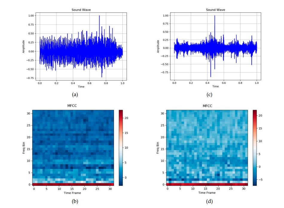
The waveform of snoring sound (a) and its MFCC spectrogram (b) compared with the waveform of the toilet flush sound (c) and corresponding MFCC image (d). Source: A Deep Learning Model for Snoring Detection (Electronic Journal, Vol.8, Issue 9)
To train a model for the Sleep.ai project, our data scientists selected a set of most relevant features from both the time and frequency domains. In combination, they created rich profiles of grinding and snoring sounds.
Selecting and training machine learning models
Since audio features come in the visual form (mostly as spectrograms), it makes them an object of image recognition that relies on deep neural networks. There are several popular architectures showing good results in sound detection and classification. Here, we only focus on two commonly used to identify sleep problems by sound.
Long short-term memory networks (LSTMs)
Long short-term memory networks (LSTMs) are known for their ability to spot long-term dependencies in data and remember information from numerous prior steps. According to sleep apnea detection research, LSTMs can achieve an accuracy of 87 percent when using MFCC features as input to separate normal snoring sounds from abnormal ones.
Another study shows even better results: the LSTM classified normal and abnormal snoring events with an accuracy of 95.3 percent. The neural network was trained using five types of features including MFCCs and short-time energy from the time domain. Together, they represent different characteristics of snoring.
Convolutional neural networks (CNNs)
Convolutional neural networks lead the pack in computer vision in healthcare and other industries. They are often referred to as a natural choice for image recognition tasks. The efficiency of CNN architecture in spectrogram processing proves the validity of this statement one more time.
In the above-mentioned project by the School of Engineering (Eastern Michigan University) a CNN-based deep learning model hit an accuracy of 96 percent in the classification of snoring vs non-snoring sounds.
Almost the same results are reported for the combination of CNN and LSTM architectures. The group of scientists from the Eindhoven University of Technology applied the CNN model to extract features from spectrograms and then run the LSTM to classify the CNN output into snore and non-snore events. The accuracy values range from 94.4 to 95.9 percent depending on the location of the microphone used for recording snoring sounds.
For Sleep.io project, the AltexSoft data science team used two CNNs (for snoring and grinding detection) and trained it on the TensorFlow platform. After models achieved an accuracy of over 80 percent, they were launched to production. Their results have been constantly getting better with the growing number of inputs collected from real users.
Building an app for snore and teeth grinding detection
To make our sound classification algorithms available to a wide audience, we packaged them into an iOS app Do I Snore or Grind, which you can freely download from the App Store. Our UX team created a unified flow enabling users to record noises during sleep, track their sleep cycle, monitor vibration events, and receive information on factors impacting sleep and tips on how they can adjust their habits. All audio data analysis is performed on-device, so you’ll get results even if there is no Internet connection. 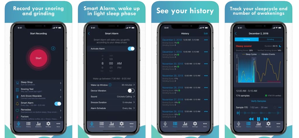
Do I Snore or Grind App interface
Keep in mind, though, that no health app, however smart it is, can replace a real doctor. The conclusion made by AI must be verified by your dentist, physician, or another medical expert.
If you want to know even more details, read our case studies
AltexSoft & Bruxlab: Employing State-of-the-Art Machine Learning and Data Science to Diagnose and Fight Bruxism
AltexSoft & SleepScore Labs: Building an iOS App for Snoring and Teeth Grinding Detection