Choosing the machine learning path when developing your software is only half the battle. Yes, it’s an advanced way of doing things. Yes, it brings automation, so widely discussed machine intelligence, and other awesome perks. But just because you put it there doesn’t guarantee your project will do well and pay off. So, how would you measure the success of a machine learning model? Various machine learning models — whether these are simpler algorithms like decision trees or state-of-the-art neural networks — need a certain metric or multiple metrics to evaluate their performance. They will help you find the pain points of your model early on and decide whether the whole ML project returns the investments and effort put into it.
In this post, we’ll examine the major machine learning metrics, explain what they are, and give recommendations on how to track them. Let’s dive in.
Machine learning pipeline in a nutshell
Before we start with metrics, it’s worth recalling the machine learning pipeline for further understanding of when the model has to be tested and evaluated and why.
Machine learning pipeline
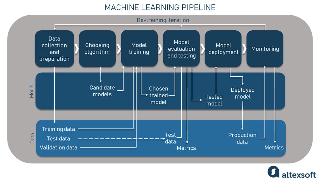
The typical machine learning model preparation flow consists of several steps. The first ones involve data collection and preparation to ensure it’s of high quality and fits the task. Here, you also do data splitting to receive samples for training, validation, and testing. Then you choose an algorithm and do the model training on historic data and make your first predictions.
The evaluation steps come after the candidate model(s) is/are trained: You test the models and measure their performance on unseen (test) data and use metrics to do that. Having compared the results, you can fine-tune it in case it doesn’t do well or send it right away to the deployment phase where end users can generate predictions on live data.
The deployed model must be continuously monitored and tested on production data to make sure that it's adequate for the current reality. The performance metrics can be applied here too to track the possible degradation of the model and capture any harmful changes so that you can re-train it on new data.
But applying metrics here is only possible if the deployed model has both predicted and ground truth data. Take, for example, a demand forecasting model for a taxi service predicting the number of people requesting a ride at 6 pm on Friday downtown. In this case, the service will receive ground truth data at 6 pm to check whether the predicted demand matched the real one. But sometimes, acquiring ground truth from production data is difficult like with sentiment analysis or image recognition cases when users don’t always have the ability to leave feedback.
In this article, we’re going to focus on the stages where tech ML metrics find their use.
What are performance metrics in machine learning?
Machine learning metrics help you quantify the performance of a machine learning model once it’s already trained. These figures give you an answer to the question, “Is my model doing well?” They help you do model testing right.
Example of how testing works
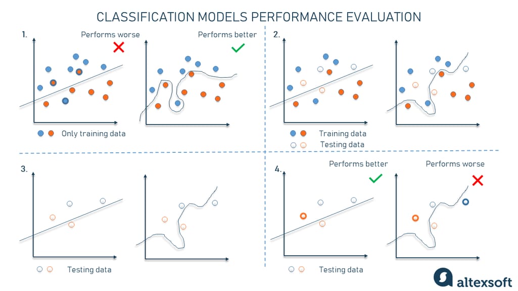
So, let’s say you have a simple binary classification task where the model needs to classify data points by color into blue and orange ones. This data lies within the 2D space. To solve this task, we can use a simpler linear regression and draw a straight line between the two classes with some orange and blue points being out of their class. Or we can opt for a more complex way of drawing boundaries between the data dots with a curved line called a higher-degree polynomial.
Why evaluating model performance is important
At first glance, it seems that the higher-degree polynomial function is a better model because it gets all the blue points on one side and all the orange points on the other one.
But is it really so? Let’s see.
Instead of using all the data as training data, we’re going to split it into two sets — one for training and one for testing. The model is trained on the portion of labeled data where classes to be predicted are already shown and the input is mapped to the output (loss function). By the way, don't confuse a loss function with metrics because the former is used to measure how the model performs during training.
Then we forget about the training set and evaluate how each model performs on the testing data. And here’s when things get changed. The linear model makes only one mistake while the higher-degree polynomial model fails two times, meaning the former does better. And you wouldn’t find that out without testing them.
But there’s still the question, “How exactly do we test a model and measure its performance?” And that’s when the metrics enter the game. Once the model is trained, these are metrics that help you figure out if it’s good or not.
Types of machine learning metrics
There are quite a few metrics out there to evaluate ML models in different applications. Most of them can be put into two categories based on the types of predictions in ML models.
Classification is a prediction type used to give the output variable in the form of categories with similar attributes. For example, such models can provide binary output such as sorting spam and non-spam messages.
Some of the popular classification metrics we’re going to cover are
Accuracy,
Precision,
Recall, and
F1 Score, etc.
Regression is a kind of prediction where the output variable is numerical, not categorical (as opposed to classification). The output is continuous. For example, it can help with predicting a patient’s length of stay in a hospital.
Some of the popular regression metrics we’re going to cover are
MSE (Mean Squared Error),
RMSE (Root Mean Squared Error), and
MAE (Mean Absolute Error).
Depending on the use case, using a single metric may not provide you with the complete picture of the problem you are solving. So, you may want to use a few metrics to better evaluate your models.
Performance metrics for classification problems
F1 Score, Accuracy, and Precision walk into a bar and say, “We’ll have some true positives and true negatives, please.” The bartender looks at them and asks, “Should I add any false negatives and false positives?”
This is an attempt at a joke. In reality, if the bartender doesn’t work as a data scientist part-time, the answer would be the typical, “Who the heck are you?”
Okay, jokes aside, the above-mentioned barflies are classification-related metrics and the drinks they ordered are predicted and actual class values within something known as the confusion matrix. But let’s dive into metrics used for machine learning classification tasks.
Confusion matrix
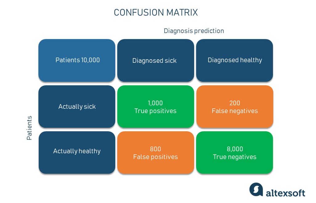
The confusion matrix is a core element that can be used to measure the performance of the ML classification model but it’s not considered a metric. By nature, it is a table with two dimensions showing actual values and predicted values. Say, we need to make a classifier that diagnoses patients as sick and healthy.
Confusion matrix example
Furthermore, both dimensions have such class instances as:
True Positive (TP) — a class is predicted true and is true in reality (patients that are sick and diagnosed sick);
True Negative (TN) — a class is predicted false and is false in reality (patients that are healthy and diagnosed healthy);
False Positive (FP) — a class is predicted true but is false in reality (patients that are healthy but diagnosed sick); and
False Negative (FN) — a class is predicted false but is true in reality (patients that are sick but diagnosed healthy).
Let’s get closer to the metrics.
Accuracy
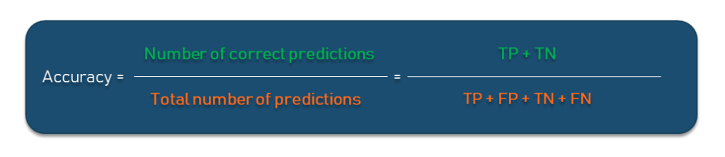
What does it show? Accuracy is used to calculate the proportion of the total number of predictions that were correct. It is the number of correct predictions divided by the total number of predictions.
Why use it? Being one of the most common classification metrics, accuracy is very intuitive and easy to understand and implement: It ranges from 0 to 100 percent or 0 to 1. If you deal with simple modeling cases, accuracy may be helpful. Besides, you can find it within any ML library like Scikit-learn for any classification model with a score method.
If we take out the healthy/sick diagnosis model, out of all 10,000 patients, the model correctly classified 9,000 patients or 90 percent or 0.9 if we measure within the range from 0 to 1. So, that’s our accuracy number.
Important to understand. While being intuitive, the accuracy metric heavily relies on data specifics. If the dataset is imbalanced (the classes in a set are presented unevenly), the result won’t be something you can trust. For example, in the training set, you have 98 percent samples of class A (healthy patients) and only 2 percent samples of class B (sick patients). The model can easily give you 98 percent training accuracy by simply predicting every patient is healthy even if they have a serious disease. Needless to say that such skewed results may have bad consequences as people won’t get needed medical help.
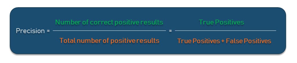
Precision
What does it show? Precision shows what proportion out of all positive predictions was correct. To calculate it, you divide the number of correct positive results (TP) by the total number of all positive results (TP + FP) predicted by the classifier.
Getting back to our example, out of all patients the model diagnosed as sick, how many did it classify correctly? We divide the number of 1,000 actually sick and predicted sick patients by the total number of those who are really sick and diagnosed sick (1,000) and those who are healthy but diagnosed sick (800). The precision result is 55.7 percent.
Why use it? Precision does well in cases when you need to or can avoid False Negatives but can’t ignore False Positives. A typical example of this is a spam detector model. It’s kind of okay if the model sends a couple of spam letters to the inbox, but sending an important non-spam email to the spam folder (False Positive) is much worse.
Important to understand. Precision is your go-to evaluation metric when dealing with imbalanced data. But it’s not a silver bullet as there are cases when false negatives and true negatives should be taken into account. For example, when it’s important to know how many actually sick people were classified as healthy and left without help.
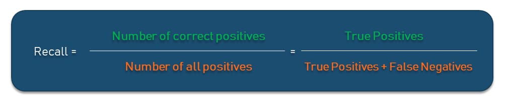
Recall
What does it show? Recall shows a proportion of correct positive predictions out of all positives a model could have made. To calculate it, you divide all True Positives by the sum of all True Positives and False Negatives in the dataset. In this way, recall provides an indication of missed positive predictions, unlike the precision metric we explained above.
In our example, it answers the question, “Out of all actually sick people, how many did the model diagnose as sick correctly?” So, following the formula, you’ll get 83.3 percent of the model's correct predictions of all positives. The closer recall to 1, the better your model is as it doesn’t miss any true positives.
Why use it? In our model, you want to find all sick people so it’s okay if the model diagnoses some healthy people as sick. They would probably be sent to take some extra tests, which is annoying but not critical. But it’s much worse if the model diagnoses some sick people as healthy and sends them home with no treatment. The recall metric does better in this case than precision as it increases the number of people with illnesses being predicted correctly and receiving their treatment.
Important to understand. Just like precision, the recall metric isn’t a one-size-fits-all solution. If we take the spam detector example, it will provide fewer correct predictions than precision.
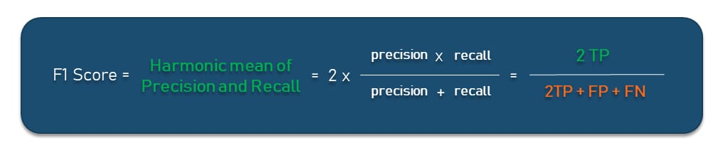
F1 Score
What does it show? The F1 Score tries to find the balance between precision and recall by calculating their harmonic mean. It is a measure of a test’s accuracy where the highest possible value is 1. This indicates perfect precision and recall.
Why use it? Some may think that to balance precision and recall, we can simply opt for the average of the results. While this can be a way, there’s a decent chance of getting a false prediction accuracy. The F1 Score is a more intricate metric that allows you to get results closer to reality on imbalanced classification problems. For example, in our medical model, the average is 69.5 percent while the F1 Score is 66.76 percent.
Important to understand. As opposed to a high F1 Score, the low one isn’t too informative: It only tells you about performance at a threshold. With it, you won’t understand whether it is a recall error or a precision error.
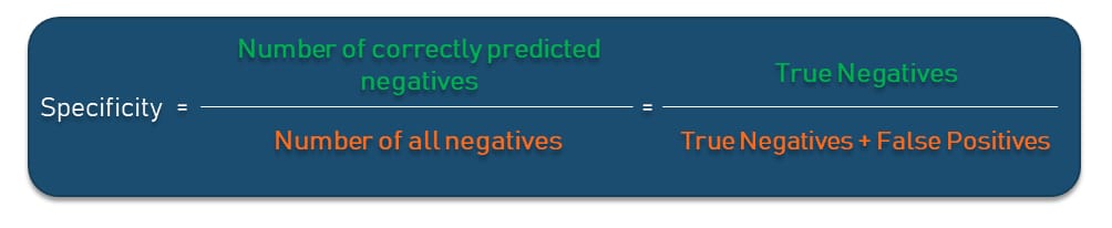
Specificity
What does it show? Specificity is the proportion of actual negatives that the model has correctly identified as such out of all negatives. It shows the True Negative Rate that is calculated as all True Negatives divided by the sum of True Negatives and False Positives in the dataset. In our matrix, specificity answers the question, “Out of all actually healthy people, how many did the model predict correctly?” Specificity is basically the opposite of recall.
Why use it? Specificity should be your metric of choice if you must cover all true negatives and you can’t tolerate any false positives in the result. Let’s take a different example which we’re going to exaggerate a bit for the showcase. Say, you’re making a fraud detection model in which all people whose credit card activity has been flagged as fraudulent (positive) will immediately go to jail. Of course, you don’t want to put any innocent person behind bars, meaning false positives here are unacceptable.
Important to understand. As with other metrics we’ve mentioned, you want your specificity score to be as close to 0 as possible. In our example, the specificity result is 8,000 * (8,000 + 200) ≅ 0.97, which is a pretty good score but still not perfect. Depending on the case, this may or may not be acceptable.
These are the most widely used classification-related metrics. There are dozens of other metrics that can be applied to measure the performance of the ML classifier, but we simply can’t review all of them in one article.
Performance metrics for regression problems
Here comes another fun part: metrics that are used to evaluate the performance of regression models. Unlike classification, regression provides output in the form of a numeric value, not a class, so you can’t use classification accuracy for evaluation. Metrics for regression involve calculating an error score to summarize the predictive skill of a model — how far the model’s predictions are from actual data values or ground truth data.
The applications of regression vary from price prediction to stock market prediction to weather forecasting. So, using the metrics to ensure that models perform well is super important here.
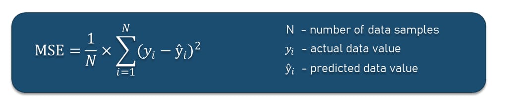
Mean Squared Error (MSE)
What does it show? Probably the most common metric for regression problems, MSE or Mean Squared Error of prediction aims at finding the average squared error between the actual values and predicted values.
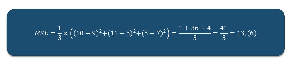
Let’s say we build a deep learning regression model to predict the number of days a particular patient will spend in a hospital. Those days a patient actually spent in a hospital are denoted as yᵢ, while the predicted amount we show with ŷᵢ. The MSE for three patients will be as follows.
Assuming we have actual data that patient A spent 10 days in a hospital, patient B spent 11 days, and patient C — 5 days with the predicted data values of 9, 5, and 7 respectively, the MSE for this model will be 13.(6). The error number is quite big considering our task. Such a result flags that the model needs to be improved.
The smaller the MSE value, the higher the accuracy of the prediction model for describing the data.
Why use it? MSE is good for optimizing the model and is easy to compute. The MSE number is an indicator for data scientists who want to improve the predictive power of the model as they can compare the MSE of each iteration, choosing the equation that generates the smallest error in the predictions.
Important to understand. MSE in general is more sensitive to outliers — data points that significantly deviate from the regular distribution of values in data. Due to squaring errors, the model can be penalized more if it makes predictions that greatly differ from the corresponding actual value. If the model deals with tasks where extreme outliers must be noticed, it’s a good idea to choose MSE as a metric because it will definitely notice them. Say, you are building a demand forecasting model for a retailer whose goods have short expiration terms. Such retailers can't allow themselves to have too many or too few goods in-store. MSE will help you find larger errors eliminating a deficit or surplus situation.
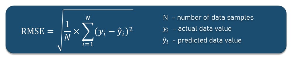
Root Mean Squared Error (RMSE)
What does it show? RMSE or Root Mean Squared Error is the extension of MSE that allows you to get rid of the squared error by calculating the square root of the MSE result.
Why use it? Sometimes we have issues with MSE because of the squared units. For example, if you build a model that predicts the price of an airline ticket in dollars, the MSE error score will have the unit “squared dollars.” This may affect the effectiveness of the model performance interpretation. RMSE, on the other hand, will have the unit “dollars” just like the target variable by taking the square root of MSE.
Important to understand. As with MSE, a perfect RMSE value is 0.0 or close to it, which means that all predictions matched the expected values exactly. But that’s rarely the case. Besides, it also isn’t robust for outliers.
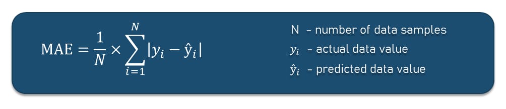
Mean Absolute Error (MAE)
What does it show? MAE or Mean Absolute Error is the average of the difference between the actual values and predicted values. It simply provides the measure of how far the predictions made by a model were from the actual output.
Why use it? Since MAE doesn’t square the error, it doesn’t give more and less weight to larger errors vs smaller errors, unlike MSE or RMSE. In cases when larger errors don’t play a significant role in a result, MAE can be a great solution. For example, for an electronics retailer, having a deficit or surplus of 10 units because the model forecasted 10 units more and less that would be sold is not a big problem. So, noticing huge and small errors in your demand forecasting model isn’t a must.
If we take the above-mentioned example with three patients, the MAE will be 3, which is a pretty good result just like RMSE’s 3.7 since they are closer to zero than the MSE number. And as we know the smaller the error number, the better the model performs. So, is it a perfect metric? No.
Important to understand. With MAE, we just get the average absolute error across all values. Since absolute is a math function that simply makes a number positive, the difference between expected and predicted — whether it is positive or negative — is always forced to be positive when calculating the MAE. Just like MSE and RMSE, its result is from 0 to infinity.
Although these three guys are the most commonly used metrics for regression, the list of other ones is quite extensive. Check, for example, what regression metrics are supported by the Scikit-learn Python machine learning library.
How to track machine learning evaluation metrics
Having dealt with the types of metrics, the next question will be how to track them to improve the model in case it doesn’t perform as planned. Here’s the rule you must remember, “If you don’t measure it, you can’t improve it.” But it’s easy to get lost in the ocean of metrics. So, here are a few recommendations on how to keep track of metrics in your machine learning project.
Measure only what matters for your particular case. Since multiple metrics are used to measure the performance of a certain machine learning model, it may be tempting to try them all. While it is still better to hold to more metrics than you think you need, don’t overdo it.
Track metrics after each iteration. If you are training models that require a lot of time and many iterations, it's better to track metrics after each iteration to see how the model does.
Use performance charts. While confusion matrices and charts are not considered metrics, they can still be helpful to understand if and how your model has improved.
Use tools to do ML monitoring in production. There are a plethora of ML model monitoring platforms capable of tracking metrics, boosting the observability of your project, and troubleshooting occurring problems. These are tools like Amazon SageMaker Model Monitor, Neptune, Censius, and many others.