

Every program relies on data and algorithms. Algorithms are sets of instructions that dictate how data is processed to produce meaningful results. Data, on the other hand, represents the information that algorithms operate on. Together, they form the foundation on which all software systems are built. Data structures play a crucial role in the interaction between algorithms and data.
This article explores the fundamentals of data structures and how they function, showing the differences between various types with examples. Whether you're just starting out or looking to enhance your programming skills, this article will equip you with the knowledge needed to navigate the complexities of data structures.
What is data structure?
Data structure is a specialized format for organizing, processing, retrieving, updating, and storing data. Data structures serve as frameworks for arranging data for specific needs or objectives. They not only store the actual data values but also maintain information about how those values are related to each other.
There are three main characteristics of a data structure that developers and data experts consider: correctness, time complexity, and space complexity.

Characteristics of a data structure
Correctness refers to the accuracy and reliability of the data structure's implementation. It should perform operations as expected, handle edge cases, and produce the right results.
Time complexity is the efficiency of data structure operations in terms of the time required to perform them. It helps us understand how the runtime of an operation grows as the input size increases.
Space complexity relates to the amount of memory an algorithm requires to perform its tasks efficiently on a particular data structure. Ideally, data structures should use as little memory as possible. This is particularly important in resource-constrained environments or when dealing with large datasets.
Balancing these characteristics is essential for selecting data structures that meet the performance requirements and maintain accuracy and reliability in all scenarios.
Data structure types
This section will discuss the main data structure types, explaining their classification and functionalities. Check out the graph below to better understand how data structure types are categorized.
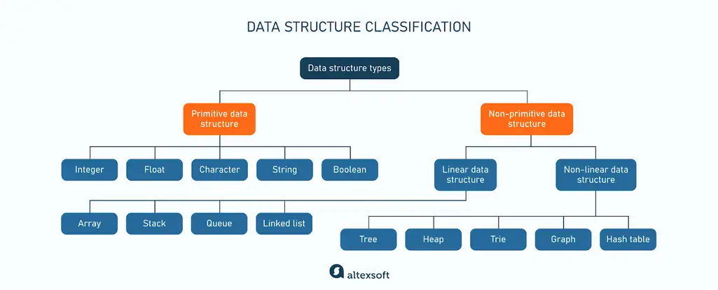
Primitive data structures or types are the most basic data units available in programming languages. They include
- integers: whole numbers—positive, negative, or zero, for example, 1, -30, 100, etc.;
- floats: decimal numbers with a fractional part, like 3.14, -0.5, 7.0;
- characters: individual characters, for example, “A,” “d,” and “1”;
- strings: sequences of characters; and
- booleans: binary values that can be either true or false, commonly used for conditional expressions.
Primitive data structures represent simple values that cannot be broken down further into smaller components. They have a fixed size and format, and this predictability helps optimize memory usage. Primitive data types are also consistent across various programming languages, with only slight variations in naming or specific implementations.
Non-primitive data structures are created with primitive data structures as their building blocks to efficiently organize and manage a collection of data. They can handle different data types and complex operations like searching, sorting, insertion, deletion, and more.
Non-primitive data structures fall into two large categories: linear and non linear structures.

Linear data structures vs. non linear data structures
The following sections will explain each category in more detail.
Linear data structures
In a linear data structure, the elements are arranged sequentially in a particular order at one level. Each element has one predecessor and one successor, except for the first and last elements. This arrangement allows for a single uninterrupted run or iteration through the structure, starting from one end and progressing to the other.
Linear data structures are typically straightforward and efficient for basic operations like adding, retrieving, or deleting. However, as the program becomes more complex, the limitations of this category become apparent. Even though linear data structures allow for single-run traversal, the process can still be complex as you have to visit each element one by one from the beginning. This results in a time complexity that increases linearly with the number of elements added.
Let’s look at the types of linear data structures in more detail.
Array data structure: Effective data storage and retrieval
An array stores elements at contiguous memory locations—next to each other without gaps. It’s homogeneous, meaning that all data within a structure is of the same data type (only integers, characters, or others described earlier.) Other linear data structures can be homogeneous or heterogeneous depending on the programming language and their implementation.
In an array, each element is associated with an index, a numerical identifier that indicates the element's position. Indexing begins at 0 for the first element and increments sequentially up to the array size minus one. For example, in an array of size 5, the indices range from 0 to 4, like in the picture below.

Compared to other linear structures, a key advantage here is that accessing any element takes the same time regardless of its position or the array’s size.
Depending on the programming language, arrays can be fixed or flexible in length. For example, in Java, you specify a constant size for an array, while in Python, you can create dynamic arrays.
Arrays are commonly used in algorithms that require random access to elements, such as searching and sorting. They are also effective for storing lists of information (like dates or addresses), performing mathematical computations, and image processing. Additionally, arrays serve as the foundation for more complex data structures.
Stack data structure: Managing undo and accessing recent elements
A stack operates on the principle of Last In, First Out (LIFO), where inserting and retrieving data is possible from only one end. The last element added to the stack is the first one to be removed.
Stack elements have two primary operations—push and pop. Pushing adds a new element, making it the top of the stack. Popping removes the topmost element first, exposing the next one as the new top of the stack. Regardless of the stack size, pushing or popping an element takes the same amount of time because there is always only one place to do the operation: the top of the stack.

Stacks are particularly useful for managing data when the order of operations is important and when you need to access the most recently added elements first. A clear example is undo mechanisms in text editors, where each action performed by a user is recorded as a command and pushed onto the stack. When you initiate an undo operation, commands are popped from the stack, canceling the previous actions and restoring the document to its previous state.
Queue data structure: Sequential processing of tasks or data
A queue operates on the principle of First In, First Out (FIFO), where the first element added to the queue is the first one to be removed. In this case, unlike with a stack, inserting and retrieving data is done from different ends. In a queue, the elements are added at the back (enqueue) and removed from the front (dequeue). Similar to a stack, adding and removing an element takes the same time regardless of the queue size.

Queues help process tasks or data in the order they were received. An example would be programs sending their print jobs, typically with only one printer available to process them sequentially. This printer handles each job in order, one at a time. Additionally, in event-driven programming, where events are processed as they occur, queues preserve the correct sequence of actions in the system.
Linked list data structure: Flexibility with dynamically growing data
A linked list consists of elements called nodes, each containing both data and a pointer (reference) to the next node in the sequence. The first node is called the head, and the last one has a null reference, indicating the end of the list. Each node can be placed at any available memory location, with the references between nodes enabling the traversal of the list.

Linked lists can grow or shrink in size dynamically, making them suitable for situations where the size of the data structure is not known in advance or may change. An example is a web browser history, where a webpage is represented as a node containing a reference to the next webpage visited.
Non linear data structures
Non linear data structures store elements not sequentially but rather in a hierarchical or arbitrary manner at different levels, often handling multiple connections. In such structures, you cannot traverse data in a single run.
Non linear data structures are more difficult to implement but offer better performance for complex operations. They maintain constant time and space complexity as the size of the data grows. Non-linear structures are also more memory efficient as they allow the same connections to be shared among multiple elements. This reduces memory consumption compared to linear structures, where each element is connected to only one predecessor and/or successor.
Let's dive into each type of non-linear data structure.
Tree data structure: Depicting hierarchical relationships with categories
A tree is a collection of elements (nodes) connected with edges that reflect parent-child relationships. Each node (except the root—the topmost node) has a single parent. Nodes without children are known as leaves. You’ve definitely seen this structure when looking at a family tree or organizational chart.

The image above shows a binary tree where each node has at most two children. There are also trinary trees with three children per node and n-ary trees where each node can have up to n children, with n being a fixed positive integer.
The height of a tree is the longest distance from the root to any leaf. The depth of a node is the length of the path from the root to that particular node. In other words, it is the level at which the node resides in the tree.
Trees are commonly used in databases to represent categories and subcategories and in file systems—for hierarchically organizing files and directories.
Heap data structure: Prioritizing tasks by importance
A heap is a binary tree where the topmost node always has the highest or the lowest value in the whole tree. This property is called the heap property or heap invariant. There are two types of heaps. In a min-heap, the value of each node is less than or equal to the values of its children. In a max-heap, the value of each node is greater than or equal to the values of its children.

With the heap data structure, we can implement priority queues, where elements have different importance. For example, job scheduling applications need to organize tasks based on urgency or deadline, and that’s where heaps come in handy.
Trie data structure: Efficient storage and retrieval of text strings
A trie, also referred to as a prefix tree or a keyword tree, is used for storing and retrieving a set of strings. In this structure, each node contains a character—typically, a letter of the alphabet.

A prefix is one or more characters that form the beginning part of one or more strings. For example, in the image above, b is a common prefix for the words ball and bee, while an is a prefix for ant and angel.
Tries are applied in cases where efficient storage and retrieval of strings are required, particularly when dealing with large datasets or dictionaries. A common example is autocompletion, where the trie structure allows quick suggestions based on partial input strings. In spell-checking algorithms, tries can also determine whether a given string is a valid word and can suggest corrections.
Graph data structure: Visualizing relationships in complex networks
A graph is a data structure used to represent relationships between entities. It consists of a set of nodes, also known as vertices, and each vertex connects to others through edges. One of the fundamental distinctions between graphs and trees is that graphs can contain cycles, while trees cannot. A cycle is a path in the graph that starts and ends at the same vertex, traversing edges without repeating any vertex.

The graph structure can depict complex network relationships, enabling efficient analysis and processing of interconnected data. For example, graphs can represent computer networks, molecular structures, and circuit layouts.
Hash table data structure: Streamlining searches and sorting operations
A hash table or hash map stores key-value pairs in an array. The key is a unique identifier to access or retrieve the value, which is the associated data or information.

The hash function takes a key as input and produces a unique numerical value called a hash code that serves as an index for a particular data element. This mapping process is deterministic, meaning the same key will always be hashed to the same index, facilitating rapid lookup and retrieval of values.
We use hash tables to quickly map keys to specific locations in the array. The goal of the hash function is to distribute keys appropriately across the array indices, minimizing collisions (situations where multiple keys map to the same index).
Hash tables are common in scenarios where efficient storage and retrieval of key-value pairs are required — for example, caching systems. Additionally, we employ hash tables in data processing tasks such as indexing and deduplication.
The evolution of data structures
Linear data structures emerged to address simple storage and retrieval needs, while non-linear structures became necessary to represent complex relationships and optimize algorithmic performance. With the increasing volumes of data being generated and evolving domain-specific challenges, there will be a continued focus on developing data structures that offer improved efficiency, scalability, and resilience.
Future advancements in areas like artificial intelligence, Internet of Things (IoT), blockchain, and edge computing may lead to the development of specialized data structures that cater to the unique requirements of these domains. It might involve advancements in data structure design, algorithmic optimizations, and parallel processing techniques.
Adaptability and openness to change are essential in the ever-changing field of technology. Overlooking this may result in performance bottlenecks, limited problem-solving abilities, and suboptimal solutions that are slower, consume more memory, and have poorer scalability.